Why the Model Layer Uses Granite TTM Forecasting with Residual Detection
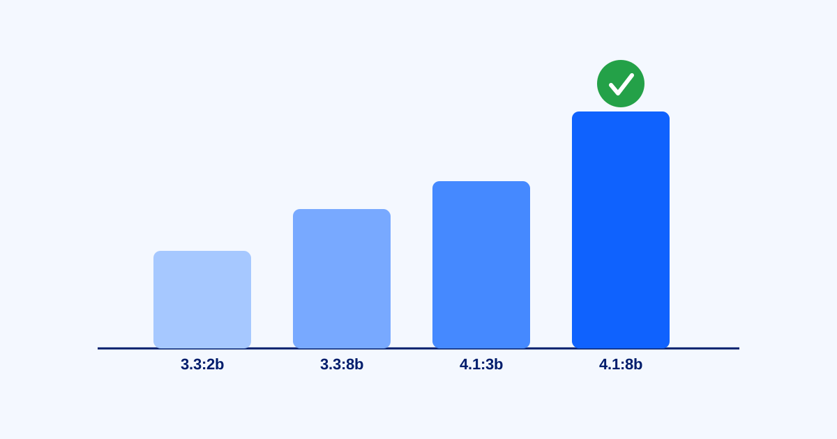
While designing the Model Layer for Granite Lifeline, we ran into a fundamental problem. The system ultimately needs to identify vehicle faults, yet most of our training data consists of unlabelled vehicle sensor readings. That makes direct fault classification difficult to train and hard to validate. Forecasting healthy vehicle behaviour gave us a practical starting point: predict what the signals should look like, compare the forecast with the observed values, and use the difference to detect anomalies.
The Question
Why does the Model Layer use Granite TTM to forecast future sensor values and then apply residual detection? Why not feed the same inputs into a classifier that outputs cooling degradation, a MAF anomaly, or an accelerator pedal sensor anomaly?
Direct classification looks simpler at first. A model receives a window of vehicle data and returns a fault type. Training that model, however, requires enough reliable fault labels to cover different vehicles, operating conditions, and levels of severity. Those labels give the classifier examples from which it can learn how each fault develops.
Our dataset does not currently provide that coverage. We therefore needed a method with a sounder training basis under the data conditions we actually have, along with outputs that we could inspect and explain.
The Problem
Our working assumption is that the available trips represent healthy vehicle operation. We reached this assumption through our review of the dataset and the information supplied with it. The data contains no confirmed fault labels that would support supervised multi-class training.
During Sprint 4, the Model Layer moved to the new feature_schema.v1. The Data Layer now supplies production_features.csv, though a set of real fault labels for multi-class classification is still unavailable.
Training a fault classifier at this stage would require labels created from hand-written rules or synthetic fault injection. A classifier trained mainly on those examples could learn the exact injection formulas we wrote, with little evidence that it had learned how faults behave in real vehicles.
Faults can also produce similar changes across related signals. MAF, MAP, engine speed, and load all interact. A deviation in one signal does not always point to a single fault type. With incomplete labels, a classifier can still return a confident category even when the evidence behind that category is weak.
For the same reason, proxy_decisions.csv remains a Data Layer responsibility in Sprint 4. The Model Layer does not treat the current healthy dataset as a complete source of fault classes.
The Options We Considered
We considered three main approaches.
The first was a direct fault classifier. Its output would be easy to consume because it could return a fault type immediately. The missing real-world labels make this difficult to train responsibly. Using synthetic faults as the main training labels would also create a high risk of overfitting to our injection design.
The second was a rules-only detector. For example, the system could raise an alert whenever coolant temperature, MAF, or pedal position crossed a fixed threshold. Rules are straightforward to implement and explain. They are less effective across different vehicles and operating conditions, and they struggle with relationships involving several signals. A fixed threshold may also flag a normal change in driving conditions as a fault.
The third was to use Granite TTM to learn healthy time-series behaviour and forecast the signals expected in the next window. The system could then calculate residuals between the forecast and the observations. A detector would use the size and duration of those residuals, together with the affected signals, to produce a risk score and a likely anomaly type.
We selected the third approach. Calibration data and targeted rules still play a role when the detector interprets the residuals.
Why We Chose Residual-Based Detection
The strongest reason was the quality of the data available to us. We have much more evidence of healthy operation than confirmed examples of faults.
Granite TTM can learn the normal relationships between signals over time from healthy trips. The model does not need a labelled example of every possible fault during forecasting. It needs to estimate how a healthy vehicle would be expected to behave under the current conditions.
When the observed signals move far enough away from that forecast, the residuals make the deviation measurable. This also gives the detector room to report weak evidence without forcing every input window into one of a few fault classes.
Residuals provide a useful explanation path. We can inspect which signal departed from its forecast, the size of that departure, how long it lasted, and how those observations contributed to the final risk score. This matters because the Model Layer passes its results to the Reasoning Layer and the dashboard.
The design also keeps forecasting and detection as separate responsibilities. Granite TTM estimates what should happen next during healthy operation. The detector measures the departure from that expectation and interprets the pattern. A future fault type can be added to the detection logic without redefining the entire forecasting task.
How This Works in the Model Layer
The Model Layer first reads production_features.csv from the Data Layer. During Sprint 4, we removed the duplicate feature computation previously carried out inside the Model Layer. The pipeline now uses the upstream features defined by feature_schema.v1, together with the calibration registry.
For each evaluation sample, Granite TTM receives 512 rows of healthy context and forecasts the following 96 rows. Once the forecast is available, the pipeline compares it with the observed values and calculates a residual for each signal.
The detector combines these residual patterns with calibration information and anomaly-specific logic. Its output includes an anomaly type, a risk score, and the signal evidence supporting the result.
The Model Layer currently focuses on three fault families:
| Fault family | Model Layer interpretation |
|---|---|
| Cooling degradation | Checks whether coolant temperature and its rate of change show a sustained departure from the healthy forecast |
| Air intake MAF anomaly | Checks MAF and related airflow features for an inconsistent pattern |
| Accelerator pedal sensor anomaly | Checks whether the relationship between pedal sensors D and E departs from its normal pattern |
Granite TTM supplies the healthy baseline. The detector then turns departures from that baseline into fault evidence.
What Sprint 4 Showed
Sprint 4 began with a comparison between zero-shot Granite TTM and a model fine-tuned on healthy trips.
With 3 epochs, a learning rate of 5e-5, and a batch size of 8, fine-tuning improved overall MAE by 4.54% over the zero-shot model. This fell short of our pre-defined 5% threshold.
Increasing the run to 5 epochs produced a 5.23% overall MAE improvement. Five of the six main signals performed at least as well as the zero-shot baseline. MAP showed a small regression of around 0.15%. The result shows that fine-tuning on healthy data improved the forecasting baseline overall, with some variation between individual signals.
We then used synthetic fault injection to test whether the residual-based detector responded to known anomalies. Each evaluation started with healthy context and introduced a fault at the forecast boundary. We used a fixed risk threshold of 0.3. A result counted as a correct detection only when the risk score reached the threshold and the reported anomaly type matched the expected type.
The initial sweep produced different results across the fault families. Cooling degradation gave the clearest response, with 11 correct detections from 11 valid samples. Weaker MAF anomalies were harder to detect, and the MAP bias control also produced mixed results. The detector can respond to injected faults, though its sensitivity still needs calibration for each anomaly family and severity level.
The experiment also clarified the relationship between forecasting and detection. A lower forecasting MAE can improve the baseline used by the detector, but it does not guarantee the same improvement in detection performance for every fault type. Forecast quality and fault detection quality are connected measures with different evaluation criteria.
Limitations
These experiments show that the detector responds to synthetic fault patterns we already know. They do not establish its performance across real vehicle faults.
The synthetic evaluation starts from healthy trips and introduces deterministic faults at a fixed point. Each sample contains one fault onset and one 96-second evaluation window. The current test does not cover intermittent faults, compound faults, degradation across several trips, or the noise and uncertainty found in data from a genuinely failing vehicle.
Performance also varies across fault families. A sustained temperature offset creates a clear residual for cooling degradation. A mild MAF or pedal sensor anomaly may sit much closer to normal driving variation. One fixed risk threshold may therefore be unsuitable across every fault type and severity level.
The current results should be read as a controlled baseline for detector sensitivity. Real-world recall and accuracy will require labelled fault data and broader validation.
What This Means Going Forward
Granite TTM forecasting with residual-based detection will remain the main Model Layer design for the current stage of the project.
Our next work is to calibrate residual scoring across anomaly types, test whether risk thresholds should vary by fault family or severity, and expand the synthetic evaluation. Intermittent faults, compound faults, and a wider range of onset positions will help us check whether the detector generalises beyond the current injection setup.
Once we have enough real fault labels, direct classification will be worth evaluating again. It may also serve as a second stage after residual detection, providing more detailed fault attribution. With the data available today, learning healthy behaviour and measuring departures from it gives us a defensible training objective, a clearer explanation path, and a design that fits the boundaries of the wider system.